Optional Lab - Regularized Cost and Gradient
Goals
In this lab, you will:
- extend the previous linear and logistic cost functions with a regularization term.
- rerun the previous example of over-fitting with a regularization term added.
import numpy as np
%matplotlib widget
import matplotlib.pyplot as plt
from plt_overfit import overfit_example, output
from lab_utils_common import sigmoid
np.set_printoptions(precision=8)
Adding regularization
The slides above show the cost and gradient functions for both linear and logistic regression. Note:
- Cost
- The cost functions differ significantly between linear and logistic regression, but adding regularization to the equations is the same.
- Gradient
- The gradient functions for linear and logistic regression are very similar. They differ only in the implementation of $f_{wb}$.
Cost functions with regularization
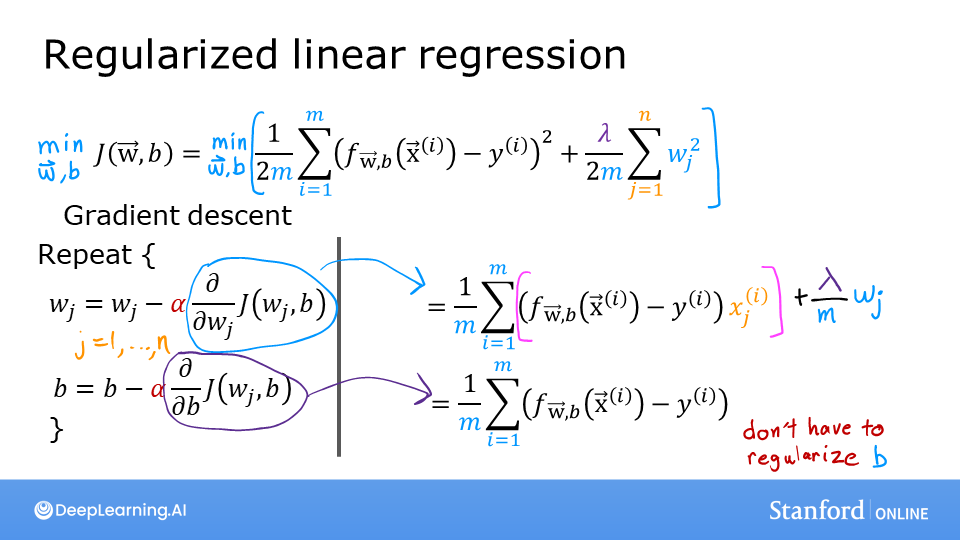
Cost function for regularized linear regression
The equation for the cost function regularized linear regression is: $$J(\mathbf{w},b) = \frac{1}{2m} \sum\limits_{i = 0}^{m-1} (f_{\mathbf{w},b}(\mathbf{x}^{(i)}) - y^{(i)})^2 + \frac{\lambda}{2m} \sum_{j=0}^{n-1} w_j^2 \tag{1}$$ where: $$ f_{\mathbf{w},b}(\mathbf{x}^{(i)}) = \mathbf{w} \cdot \mathbf{x}^{(i)} + b \tag{2} $$
Compare this to the cost function without regularization (which you implemented in a previous lab), which is of the form:
$$J(\mathbf{w},b) = \frac{1}{2m} \sum\limits_{i = 0}^{m-1} (f_{\mathbf{w},b}(\mathbf{x}^{(i)}) - y^{(i)})^2 $$
The difference is the regularization term, $\frac{\lambda}{2m} \sum_{j=0}^{n-1} w_j^2$
Including this term encourages gradient descent to minimize the size of the parameters. Note, in this example, the parameter $b$ is not regularized. This is standard practice.
Below is an implementation of equations (1) and (2). Note that this uses a standard pattern for this course, a for loop over all m examples.
def compute_cost_linear_reg(X, y, w, b, lambda_ = 1):
    """
    Computes the cost over all examples
    Args:
      X (ndarray (m,n): Data, m examples with n features
      y (ndarray (m,)): target values
      w (ndarray (n,)): model parameters
      b (scalar)      : model parameter
      lambda_ (scalar): Controls amount of regularization
    Returns:
      total_cost (scalar):  cost
    """

    m  = X.shape[0]
    n  = len(w)
    cost = 0.
    for i in range(m):
        f_wb_i = np.dot(X[i], w) + b                                   #(n,)(n,)=scalar, see np.dot
        cost = cost + (f_wb_i - y[i])**2                               #scalar
    cost = cost / (2 * m)                                              #scalar

    reg_cost = 0
    for j in range(n):
        reg_cost += (w[j]**2)                                          #scalar
    reg_cost = (lambda_/(2*m)) * reg_cost                              #scalar

    total_cost = cost + reg_cost                                       #scalar
    return total_cost                                                  #scalar
Run the cell below to see it in action.
np.random.seed(1)
X_tmp = np.random.rand(5,6)
y_tmp = np.array([0,1,0,1,0])
w_tmp = np.random.rand(X_tmp.shape[1]).reshape(-1,)-0.5
b_tmp = 0.5
lambda_tmp = 0.7
cost_tmp = compute_cost_linear_reg(X_tmp, y_tmp, w_tmp, b_tmp, lambda_tmp)

print("Regularized cost:", cost_tmp)
Expected Output:
| Regularized cost: 0.07917239320214275 |
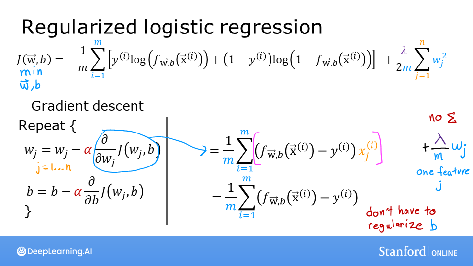
Cost function for regularized logistic regression
For regularized logistic regression, the cost function is of the form $$J(\mathbf{w},b) = \frac{1}{m} \sum_{i=0}^{m-1} \left[ -y^{(i)} \log\left(f_{\mathbf{w},b}\left( \mathbf{x}^{(i)} \right) \right) - \left( 1 - y^{(i)}\right) \log \left( 1 - f_{\mathbf{w},b}\left( \mathbf{x}^{(i)} \right) \right) \right] + \frac{\lambda}{2m} \sum_{j=0}^{n-1} w_j^2 \tag{3}$$ where: $$ f_{\mathbf{w},b}(\mathbf{x}^{(i)}) = sigmoid(\mathbf{w} \cdot \mathbf{x}^{(i)} + b) \tag{4} $$
Compare this to the cost function without regularization (which you implemented in a previous lab):
$$ J(\mathbf{w},b) = \frac{1}{m}\sum_{i=0}^{m-1} \left[ (-y^{(i)} \log\left(f_{\mathbf{w},b}\left( \mathbf{x}^{(i)} \right) \right) - \left( 1 - y^{(i)}\right) \log \left( 1 - f_{\mathbf{w},b}\left( \mathbf{x}^{(i)} \right) \right)\right] $$
As was the case in linear regression above, the difference is the regularization term, which is $\frac{\lambda}{2m} \sum_{j=0}^{n-1} w_j^2$
Including this term encourages gradient descent to minimize the size of the parameters. Note, in this example, the parameter $b$ is not regularized. This is standard practice.
def compute_cost_logistic_reg(X, y, w, b, lambda_ = 1):
    """
    Computes the cost over all examples
    Args:
    Args:
      X (ndarray (m,n): Data, m examples with n features
      y (ndarray (m,)): target values
      w (ndarray (n,)): model parameters
      b (scalar)      : model parameter
      lambda_ (scalar): Controls amount of regularization
    Returns:
      total_cost (scalar):  cost
    """

    m,n  = X.shape
    cost = 0.
    for i in range(m):
        z_i = np.dot(X[i], w) + b                                      #(n,)(n,)=scalar, see np.dot
        f_wb_i = sigmoid(z_i)                                          #scalar
        cost +=  -y[i]*np.log(f_wb_i) - (1-y[i])*np.log(1-f_wb_i)      #scalar

    cost = cost/m                                                      #scalar

    reg_cost = 0
    for j in range(n):
        reg_cost += (w[j]**2)                                          #scalar
    reg_cost = (lambda_/(2*m)) * reg_cost                              #scalar

    total_cost = cost + reg_cost                                       #scalar
    return total_cost                                                  #scalar
Run the cell below to see it in action.
np.random.seed(1)
X_tmp = np.random.rand(5,6)
y_tmp = np.array([0,1,0,1,0])
w_tmp = np.random.rand(X_tmp.shape[1]).reshape(-1,)-0.5
b_tmp = 0.5
lambda_tmp = 0.7
cost_tmp = compute_cost_logistic_reg(X_tmp, y_tmp, w_tmp, b_tmp, lambda_tmp)

print("Regularized cost:", cost_tmp)
Expected Output:
| Regularized cost: 0.6850849138741673 |
Gradient descent with regularization
The basic algorithm for running gradient descent does not change with regularization, it is: $$\begin{align*} &\text{repeat until convergence:} \; \lbrace \\ & \; \; \;w_j = w_j - \alpha \frac{\partial J(\mathbf{w},b)}{\partial w_j} \tag{1} \; & \text{for j := 0..n-1} \\ & \; \; \; \; \;b = b - \alpha \frac{\partial J(\mathbf{w},b)}{\partial b} \\ &\rbrace \end{align*}$$ Where each iteration performs simultaneous updates on $w_j$ for all $j$.
What changes with regularization is computing the gradients.
Computing the Gradient with regularization (both linear/logistic)
The gradient calculation for both linear and logistic regression are nearly identical, differing only in computation of $f_{\mathbf{w}b}$. $$\begin{align*} \frac{\partial J(\mathbf{w},b)}{\partial w_j} &= \frac{1}{m} \sum\limits_{i = 0}^{m-1} (f_{\mathbf{w},b}(\mathbf{x}^{(i)}) - y^{(i)})x_{j}^{(i)} + \frac{\lambda}{m} w_j \tag{2} \\ \frac{\partial J(\mathbf{w},b)}{\partial b} &= \frac{1}{m} \sum\limits_{i = 0}^{m-1} (f_{\mathbf{w},b}(\mathbf{x}^{(i)}) - y^{(i)}) \tag{3} \end{align*}$$
m is the number of training examples in the data set
$f_{\mathbf{w},b}(x^{(i)})$ is the model's prediction, while $y^{(i)}$ is the target
For a linear regression model
$f_{\mathbf{w},b}(x) = \mathbf{w} \cdot \mathbf{x} + b$For a logistic regression model
$z = \mathbf{w} \cdot \mathbf{x} + b$
$f_{\mathbf{w},b}(x) = g(z)$
where $g(z)$ is the sigmoid function:
$g(z) = \frac{1}{1+e^{-z}}$
The term which adds regularization is the $\frac{\lambda}{m} w_j $.
Gradient function for regularized linear regression
def compute_gradient_linear_reg(X, y, w, b, lambda_):
    """
    Computes the gradient for linear regression
    Args:
      X (ndarray (m,n): Data, m examples with n features
      y (ndarray (m,)): target values
      w (ndarray (n,)): model parameters
      b (scalar)      : model parameter
      lambda_ (scalar): Controls amount of regularization

    Returns:
      dj_dw (ndarray (n,)): The gradient of the cost w.r.t. the parameters w.
      dj_db (scalar):       The gradient of the cost w.r.t. the parameter b.
    """
    m,n = X.shape           #(number of examples, number of features)
    dj_dw = np.zeros((n,))
    dj_db = 0.

    for i in range(m):
        err = (np.dot(X[i], w) + b) - y[i]
        for j in range(n):
            dj_dw[j] = dj_dw[j] + err * X[i, j]
        dj_db = dj_db + err
    dj_dw = dj_dw / m
    dj_db = dj_db / m

    for j in range(n):
        dj_dw[j] = dj_dw[j] + (lambda_/m) * w[j]

    return dj_db, dj_dw
Run the cell below to see it in action.
np.random.seed(1)
X_tmp = np.random.rand(5,3)
y_tmp = np.array([0,1,0,1,0])
w_tmp = np.random.rand(X_tmp.shape[1])
b_tmp = 0.5
lambda_tmp = 0.7
dj_db_tmp, dj_dw_tmp =  compute_gradient_linear_reg(X_tmp, y_tmp, w_tmp, b_tmp, lambda_tmp)

print(f"dj_db: {dj_db_tmp}", )
print(f"Regularized dj_dw:\n {dj_dw_tmp.tolist()}", )
Expected Output
dj_db: 0.6648774569425726
Regularized dj_dw:
 [0.29653214748822276, 0.4911679625918033, 0.21645877535865857]
Gradient function for regularized logistic regression
def compute_gradient_logistic_reg(X, y, w, b, lambda_):
    """
    Computes the gradient for linear regression

    Args:
      X (ndarray (m,n): Data, m examples with n features
      y (ndarray (m,)): target values
      w (ndarray (n,)): model parameters
      b (scalar)      : model parameter
      lambda_ (scalar): Controls amount of regularization
    Returns
      dj_dw (ndarray Shape (n,)): The gradient of the cost w.r.t. the parameters w.
      dj_db (scalar)            : The gradient of the cost w.r.t. the parameter b.
    """
    m,n = X.shape
    dj_dw = np.zeros((n,))                            #(n,)
    dj_db = 0.0                                       #scalar

    for i in range(m):
        f_wb_i = sigmoid(np.dot(X[i],w) + b)          #(n,)(n,)=scalar
        err_i  = f_wb_i  - y[i]                       #scalar
        for j in range(n):
            dj_dw[j] = dj_dw[j] + err_i * X[i,j]      #scalar
        dj_db = dj_db + err_i
    dj_dw = dj_dw/m                                   #(n,)
    dj_db = dj_db/m                                   #scalar

    for j in range(n):
        dj_dw[j] = dj_dw[j] + (lambda_/m) * w[j]

    return dj_db, dj_dw
Run the cell below to see it in action.
np.random.seed(1)
X_tmp = np.random.rand(5,3)
y_tmp = np.array([0,1,0,1,0])
w_tmp = np.random.rand(X_tmp.shape[1])
b_tmp = 0.5
lambda_tmp = 0.7
dj_db_tmp, dj_dw_tmp =  compute_gradient_logistic_reg(X_tmp, y_tmp, w_tmp, b_tmp, lambda_tmp)

print(f"dj_db: {dj_db_tmp}", )
print(f"Regularized dj_dw:\n {dj_dw_tmp.tolist()}", )
Expected Output
dj_db: 0.341798994972791
Regularized dj_dw:
 [0.17380012933994293, 0.32007507881566943, 0.10776313396851499]
Rerun over-fitting example
plt.close("all")
display(output)
ofit = overfit_example(True)
In the plot above, try out regularization on the previous example. In particular:
- Categorical (logistic regression)
- set degree to 6, lambda to 0 (no regularization), fit the data
- now set lambda to 1 (increase regularization), fit the data, notice the difference.
- Regression (linear regression)
- try the same procedure.
Congratulations!
You have:
- examples of cost and gradient routines with regularization added for both linear and logistic regression
- developed some intuition on how regularization can reduce over-fitting